1. Home
2. Getting Started Tutorial
3. Part 5: Ad-Hoc Data Analysis

Part 5: Ad-Hoc Data Analysis

After you have loaded your tables, either manually or using a data source connector, manipulated the data in SQL, written it into Tableau BI or into GoodData BI, and set everything to run automatically, let’s take a look at some additional Keboola features related to doing ad-hoc analysis.

This part of the tutorial shows how to work with arbitrary data in Python in a completely unrestricted way. Although our examples use the Python language, the very same can be achieved using R or Julia.

Before you start, you should have a basic understanding of the Python language.

• Introduction
• Using BigQuery Connector
  • Prepare
    • Service account
    • Google Storage bucket
  • Extract Data
• Exploring Data
• Adding Libraries
  • Working with Custom Libraries
• Wrap Up
• Final Note

Introduction

Let’s say you want to experiment with the US unemployment data. It is provided by the U.S. Bureau of Labor Statistics (BLS), and the dataset A-10 contains unemployment rates by month. The easiest way to access the data is via Google Public Data, which contains a dataset called Bureau of Labor Statistics Data.

Google Public Data can be queried using BigQuery and brought into Keboola with the help of our BigQuery data source connector. Preview the table data in Google BigQuery.

Using BigQuery Connector

To work with Google BigQuery, create an account, and enable billing. Remember, querying public data is only free up to 1TB a month.

Then create a service account for authentication of the Google BigQuery data source connector, and create a Google Storage bucket as a temporary storage for off-loading the data from BigQuery.

Note: If setting up the Google BigQuery connector seems too complicated to you, export the query results to Google Sheets and load them from Google Drive. Or, export them to a CSV file and load them from local files.

Prepare

Before you start, have a Google service account and a Google Storage bucket ready.

Service account

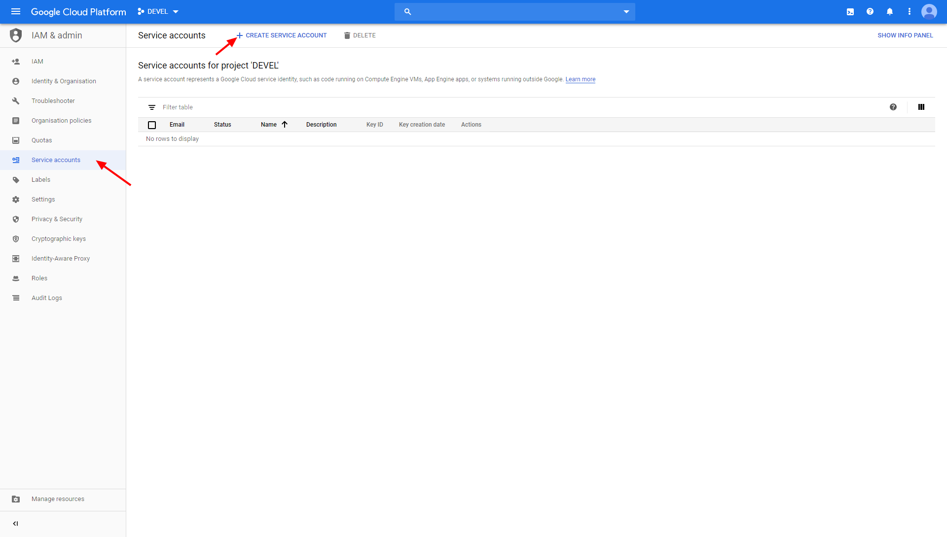
To create a Google service account, go to the Google Cloud Platform Console > IAM & admin > Service accounts and create a new service account:

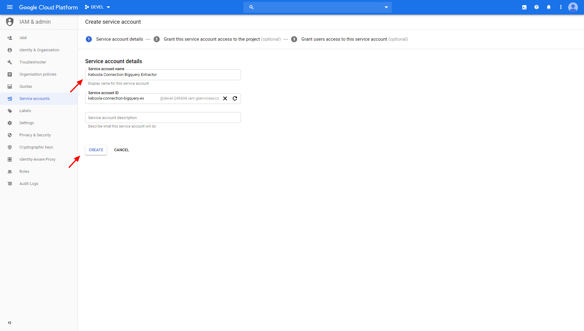
Name the service account:

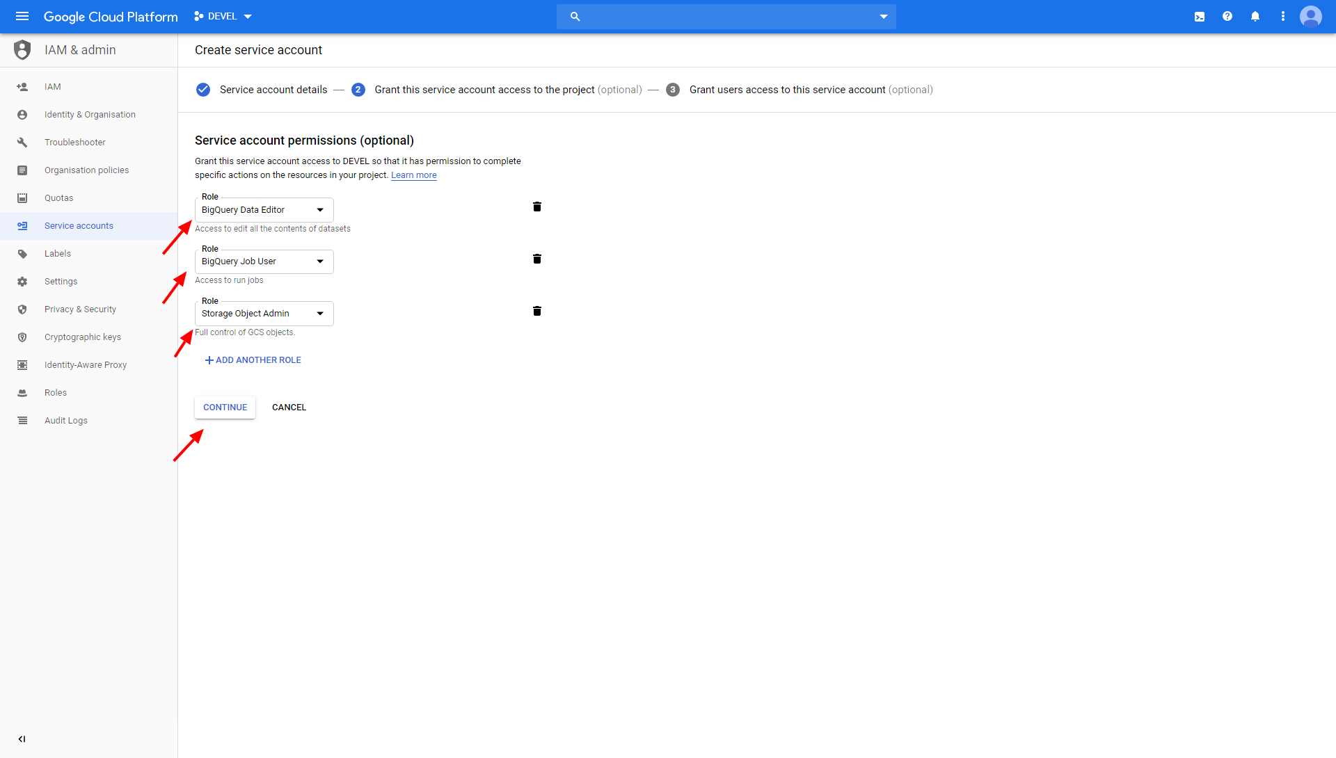
Grant the roles BigQuery Data Editor, BigQuery Job User and Storage Object Admin to your service account:

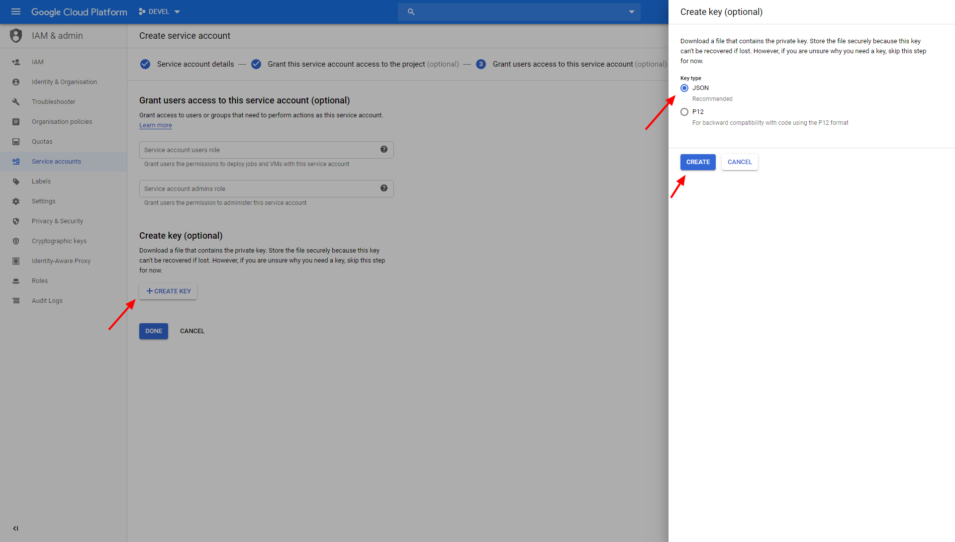
Finally, create a new JSON key and download it to your computer:

Google Storage bucket

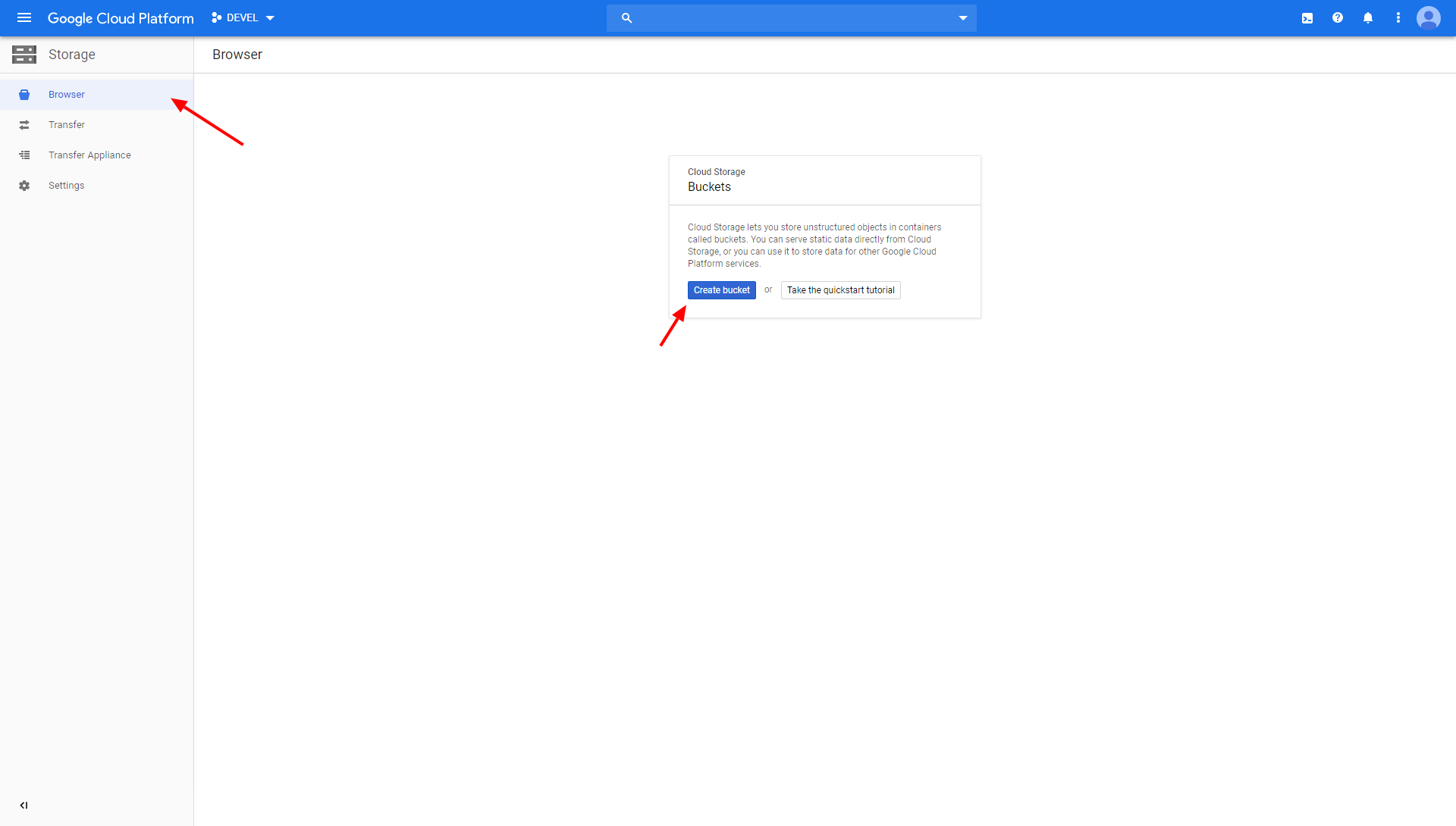
To create a Google Storage bucket, go to the Google Cloud Platform console > Storage and create a new bucket:

Enter the bucket’s name and choose where to store your data (the location type Region is okay for our purpose):

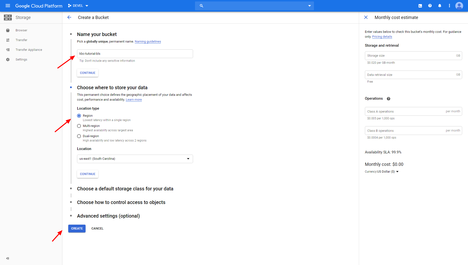
Do not set a retention policy on the bucket. The bucket contains only temporary data and no retention is needed.

Extract Data

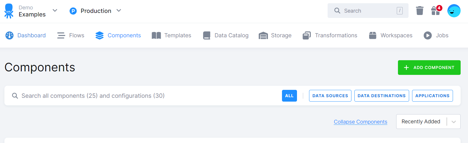
Now you’re ready to load the data into Keboola. Go to the section Components, and click the green button Add Component:

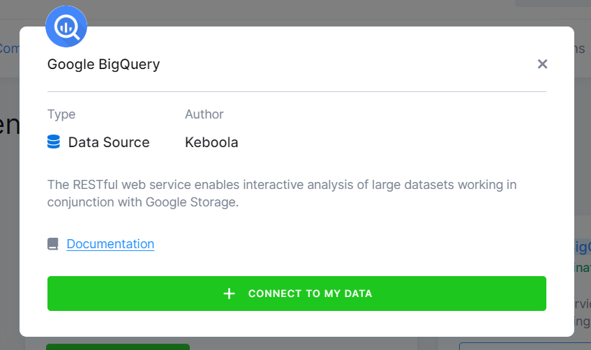
Use the search to find the Google BigQuery data source:

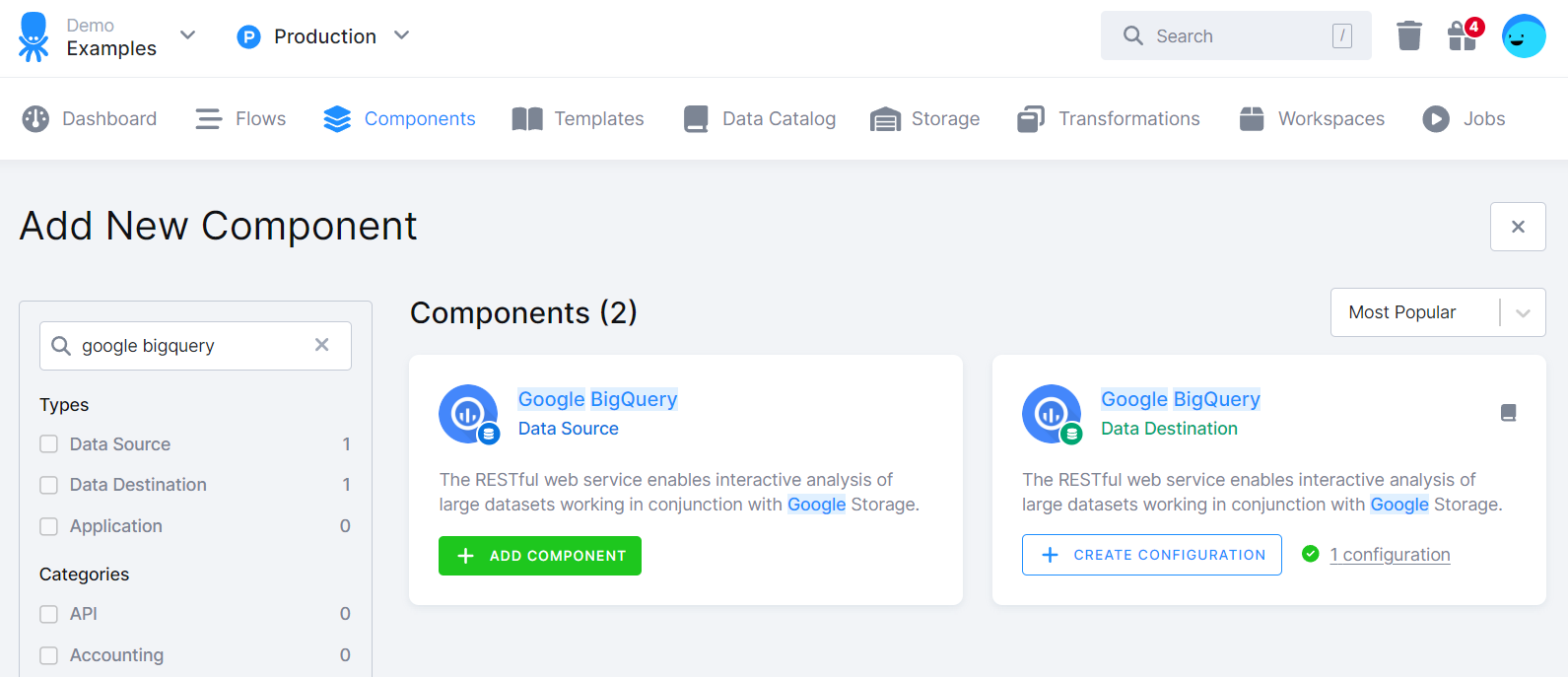
Click + Add Component and then Connect to My Data:

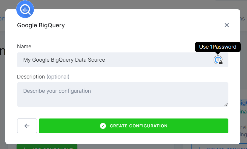
Name the configuration (e.g., ‘Bls Unemployment’) and describe it if you want. Then, click Create Configuration:

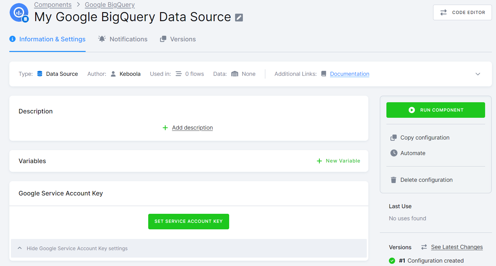
Then set the service account key:

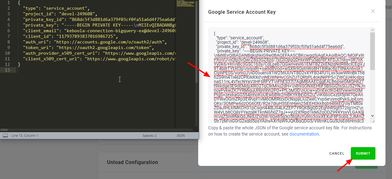
Open the downloaded key you have created above in a text editor, copy & paste it in the input field, click Submit and then Save.

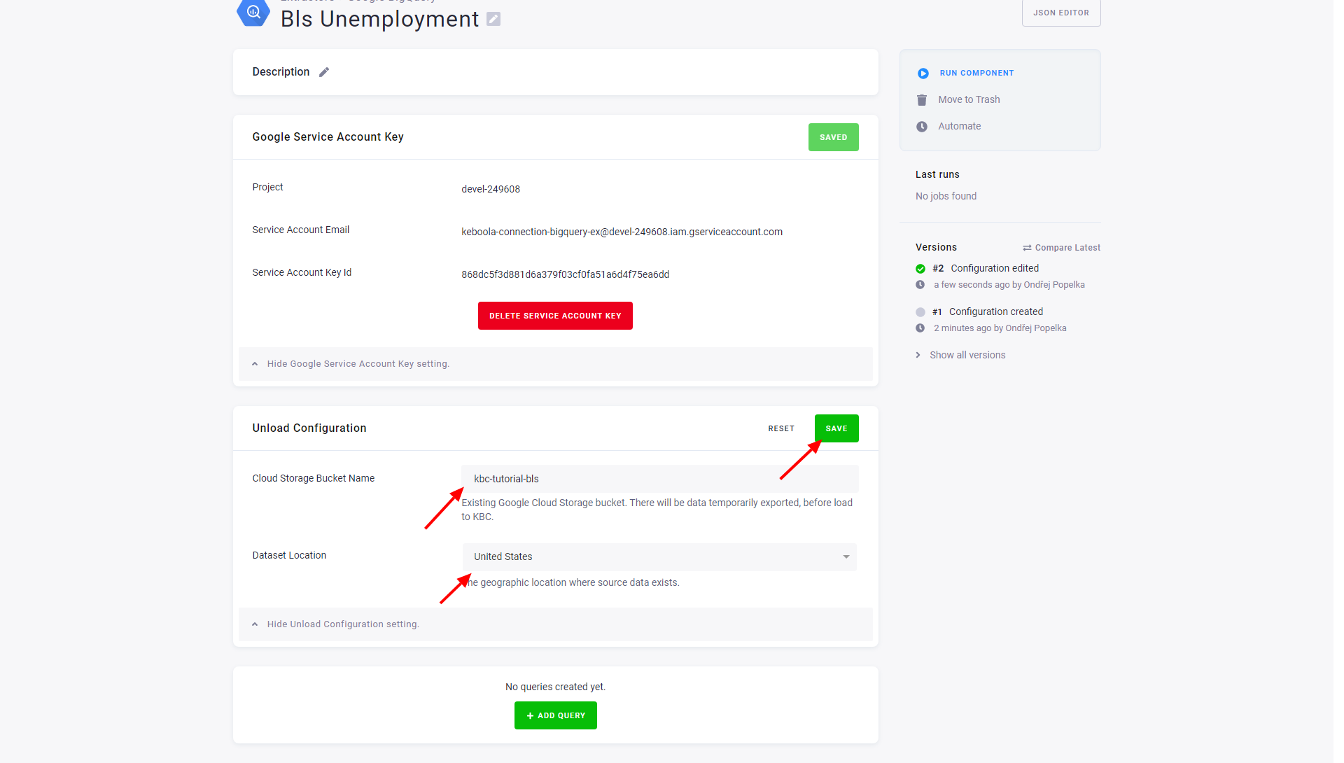
Fill the bucket you have created above:

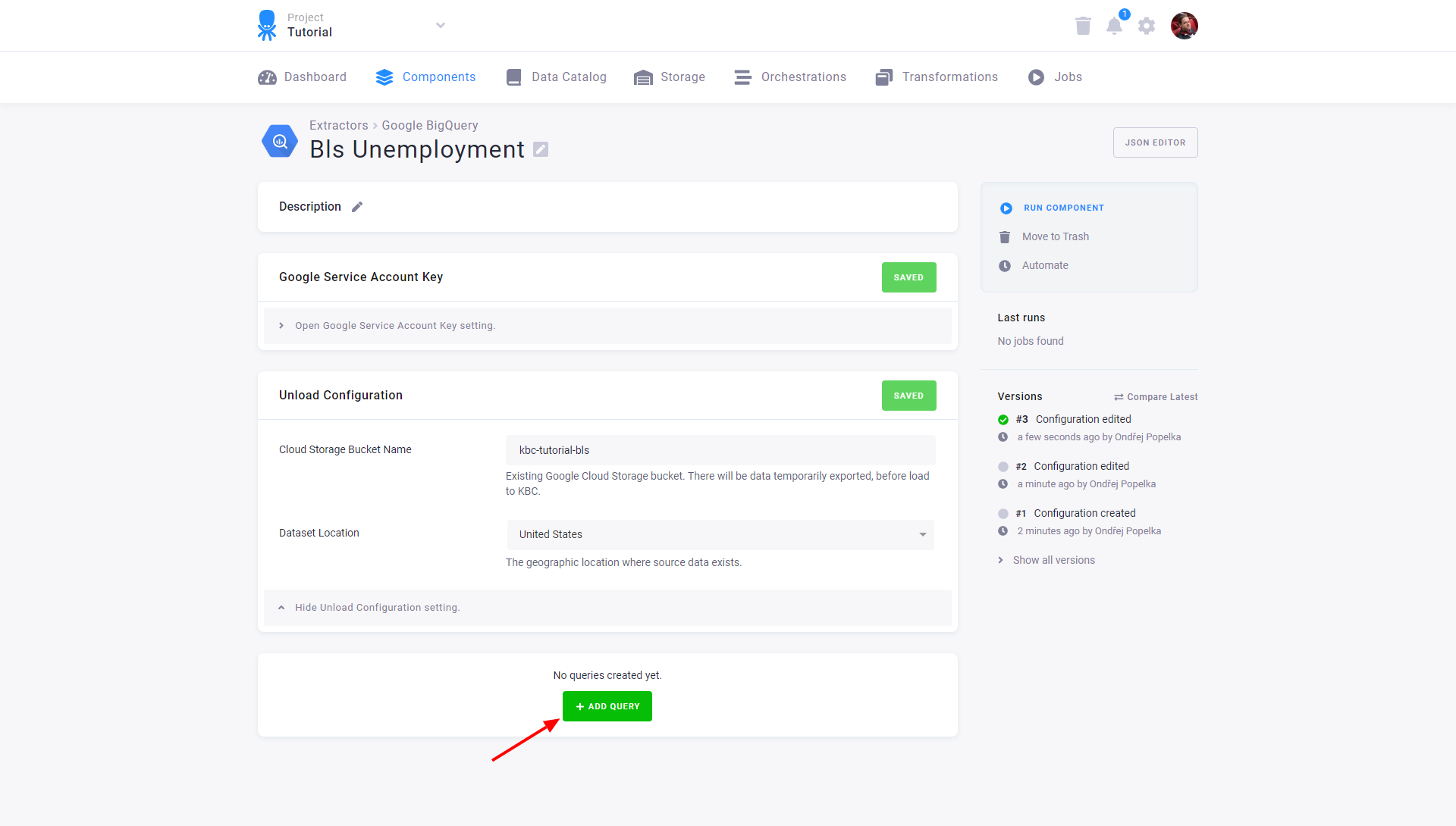
After that configure the actual extraction queries by clicking the Add Query button:

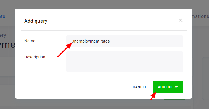
Name the query, e.g., Unemployment rates:

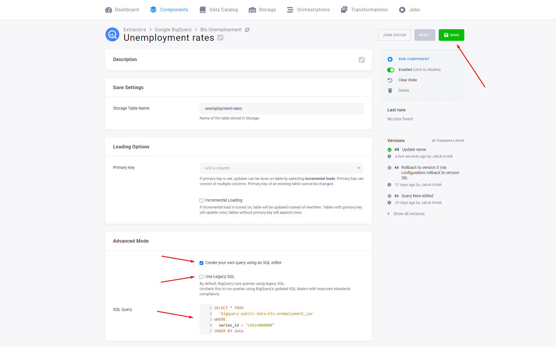
Check Create your own query using an SQL editor, uncheck the Use Legacy SQL setting, and paste the following code in the SQL Query field:

SELECT * FROM
  `bigquery-public-data.bls.unemployment_cps`
WHERE
  series_id = "LNS14000000"
ORDER BY date

The LNS14000000 series will pick the unemployment rates only.

Then Save the query configuration.

Now run the configuration to bring the data to Keboola:

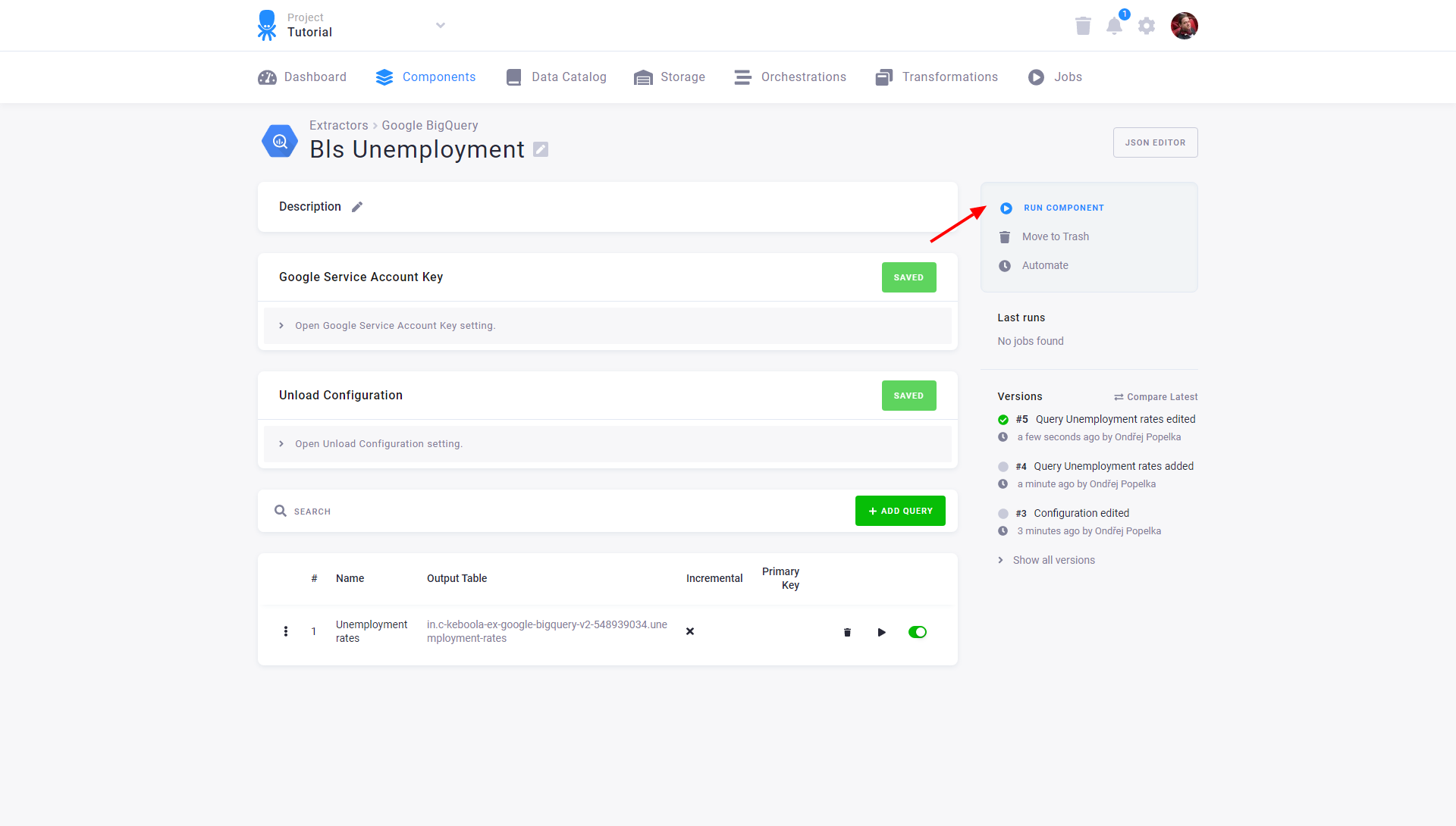
Running the data source connector creates a background job that

• executes the queries in Google BigQuery.
• saves the results to Google Cloud Storage.
• exports the results from Google Cloud Storage and stores them in specified tables in Keboola Storage.
• removes the results from Google Cloud Storage.

When a job is running, a small orange circle appears under Last runs, along with RunId and other info on the job. Green is for success, red for failure. Click on the indicator, or the info next to it, for more details. Once the job is finished, click on the names of the tables to inspect their contents.

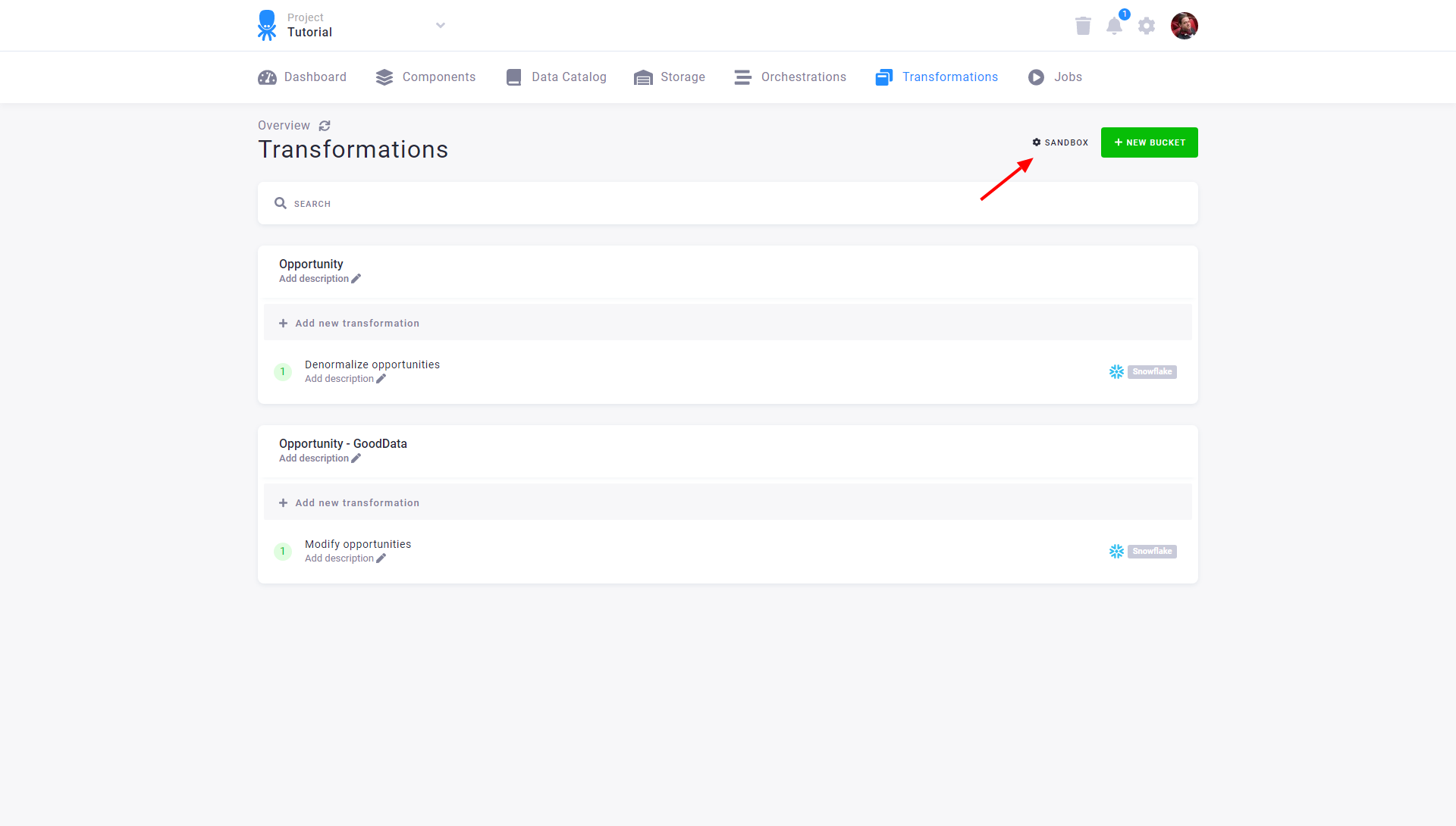
Exploring Data

To explore the data, go to Transformations, and click on Sandbox. Provided for each user and project automatically, it is an isolated environment in which you can experiment without interfering with any production code.

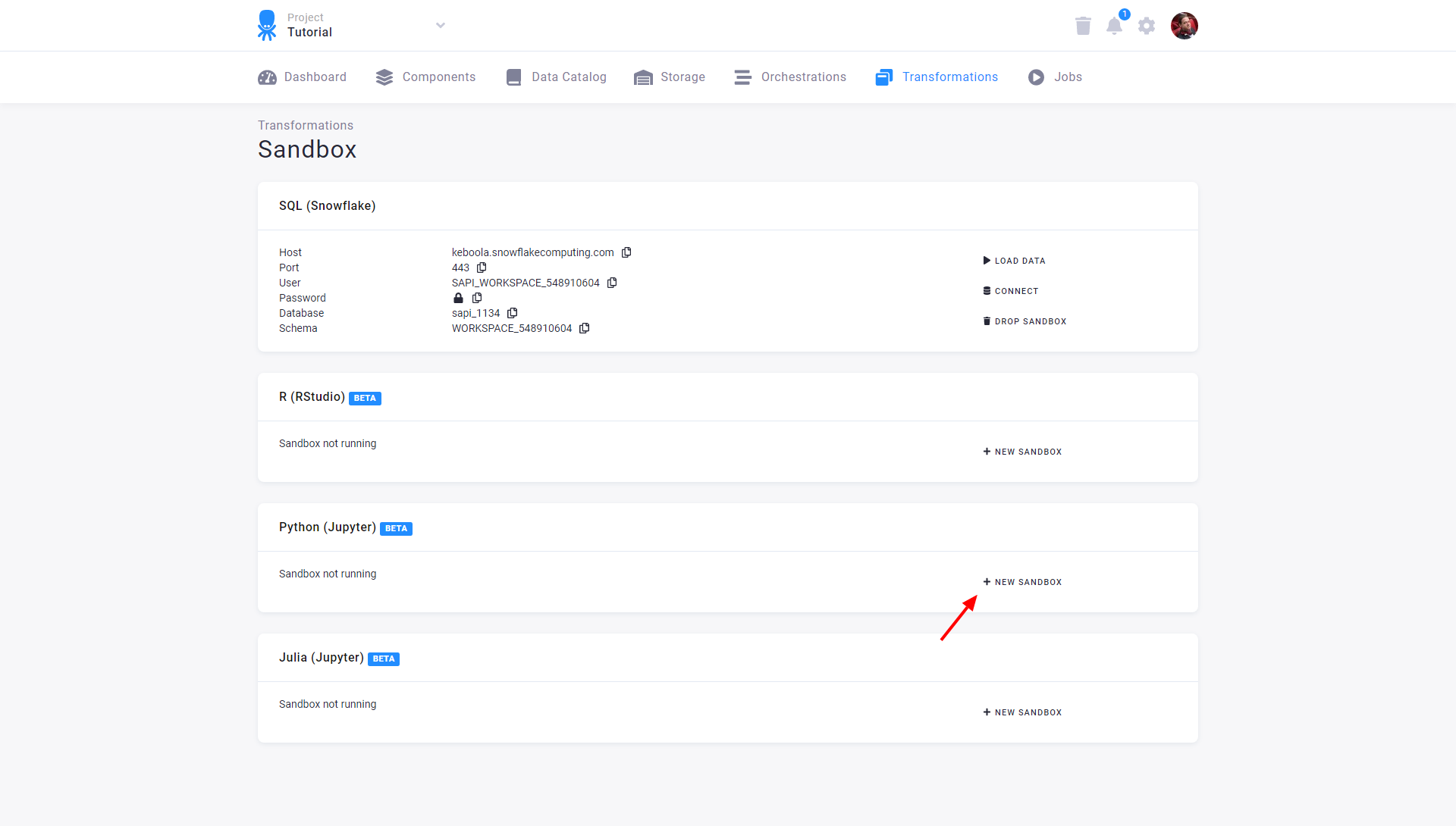
Click on New Sandbox next to Python (Jupyter):

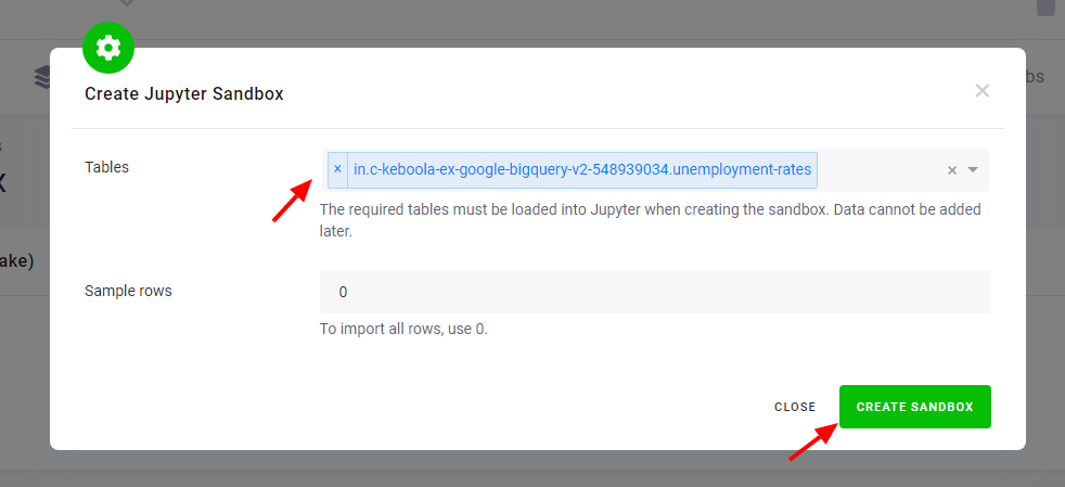
Select the unemployment rates table (in.c-keboola-ex-google-bigquery-v2-548939034.unemployment-rates in this case), click on Create Sandbox. Wait for the process to finish:

When finished, connect to the web version of the Jupyter Notebook. It allows you to run arbitrary code by clicking the Connect button:

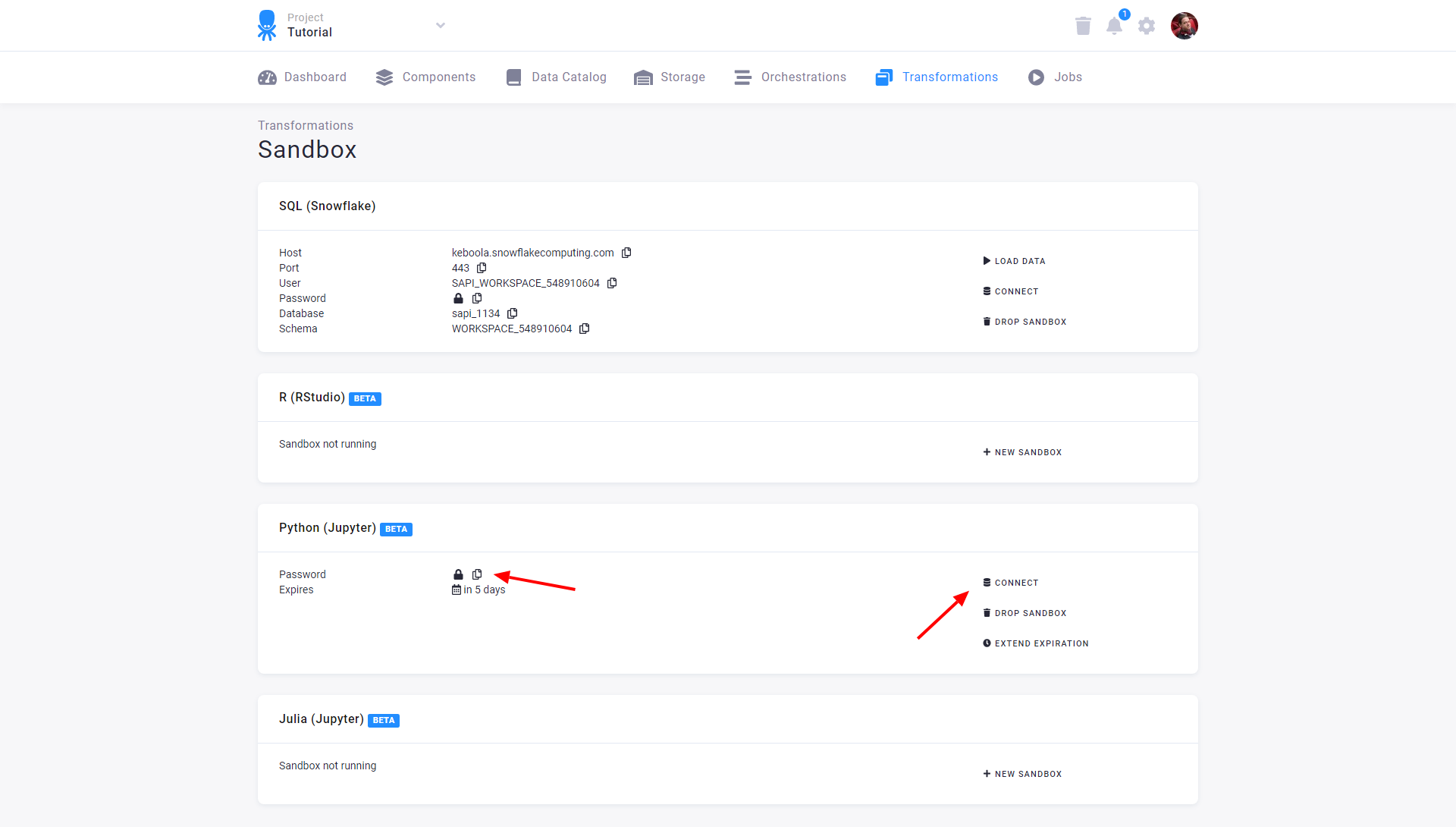
When prompted, enter the password from the Sandbox screen:

You can now run arbitrary code in Python, using common data scientist tools like Pandas or Matplotlib. For instance, to load the file, use (make sure to use the correct filename):

import pandas
df = pandas.read_csv("/data/in/tables/in.c-keboola-ex-google-bigquery-v2-548939034.unemployment-rates.csv",sep=',')
df.head()

The path /data/in/tables/ is the location for loaded tables; they are loaded as simple CSV files. Once your table is loaded, you can play with it:

import matplotlib.pyplot as plt
years = df.groupby(df['year'])['value'].mean()
years.plot(kind='line', color = 'orange')
plt.xlabel("Year")
plt.ylabel("Average %")
plt.suptitle('US Unemployment Rate', size=15)
plt.show()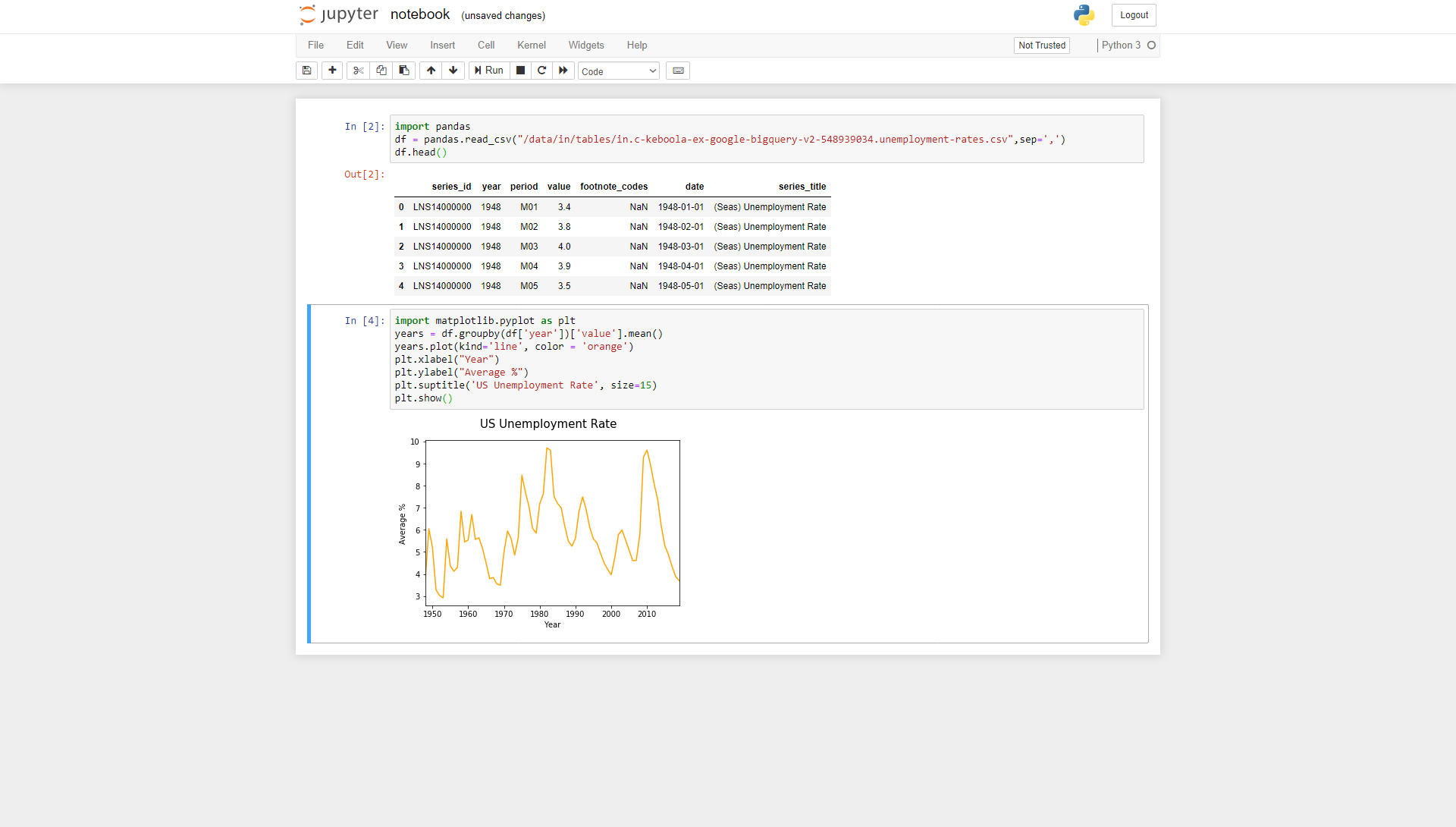

Adding Libraries

Now that you can experiment with the U.S. unemployment data extracted from Google BigQuery (or any other data extracted in any other way), you can do the same with the EU unemployment data. Available at Eurostat, the unemployment dataset is called tgs00010.

There are a number of ways how to get the data from Eurostat – e.g., you can download it in TSV or XLS format. To avoid downloading the (possibly) lengthy data set to your hard drive, Eurostat provides a REST API for downloading the data. This could be processed using the Generic Extractor. However, the data is provided in JSON-stat format, which contains tables encoded using the row-major method. Even though it is possible to import them to Keboola, it would be necessary to do additional processing to obtain plain tables.

To save time, use a tool designed for that – pyjstat. It is a Python library which can read JSON-stat data directly into a Pandas data frame. Although this library is not installed by default in the Jupyter Sandbox environment, nothing prevents you from installing it.

Working with Custom Libraries

Use the following code to download the desired data from Eurostat:

import subprocess
import sys
subprocess.call([sys.executable, '-m', 'pip', 'install', '--disable-pip-version-check', '-q', 'pyjstat'])
from pyjstat import pyjstat
dataset = pyjstat.Dataset.read('http://ec.europa.eu/eurostat/wdds/rest/data/v2.1/json/en/tgs00010?sex=T&precision=1&unit=PC&age=Y_GE15')
df = dataset.write('dataframe')
df.head()

The URL was built using the Eurostat Query Builder. Also note that installing a library from within the Python code must be done using pip install. Now that you have the data, feel free to play with it:

years = df.groupby(df['time'])['value'].mean()
years.plot(kind='line', color = 'orange')
plt.xlabel("Year")
plt.ylabel("Average %")
plt.suptitle('EU Unemployment Rate', size=15)
plt.show()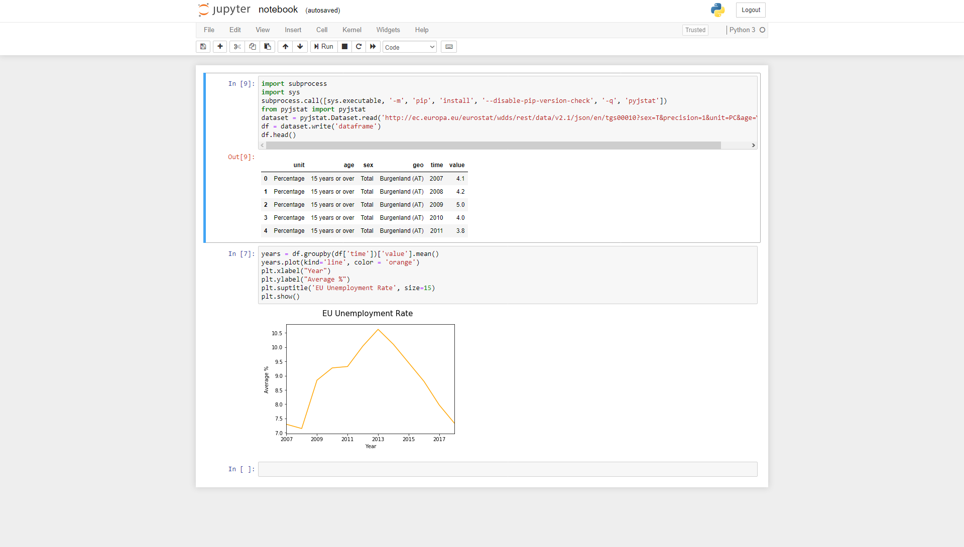

Wrap Up

You have just learnt to do a completely ad-hoc analysis of various data sets. If you need to run the above code regularly, simply copy&paste it into a Transformation.

The above tutorial is done in the Python language using the Jupyter Notebook. The same can be done in the R language using RStudio, or in Julia using Jupyter Notebook. For more information about sandboxes (including disk and memory limits), see the corresponding documentation.

Final Note

This is the end of our stroll around Keboola. On our walk, we missed quite a few things: Applications, Python, R and Julia transformations, Redshift and Snowflake features, to name a few. However, teaching you everything was not really the point of this tutorial. We wanted to show you how Keboola can help in connecting different systems together.

Return to the beginning or contact us.